The aim of a neutrino factory is to produce intense beams of neutrinos by trapping muons in a storage ring until they decay. Muons, having a half-life t˝~1.56ms, are not readily available in nature and must be produced earlier on in the accelerator system. The suggested way of doing this starts with a proton beam of several GeV and fires it at a target material, which emits pions (p+) that decay into the required muons (m+) soon afterwards (t˝~26.0ns).
The main difficulty with this scheme is that the distribution of pions emitted from the source has an extremely large emittance: in the dataset used, 22% of the pions are actually going backwards in the lab frame (vz<0), so the emittance can hardly even be calculated. This means that any simulation based on conventional assumptions about the beam's general direction and size are likely to be inappropriate. There are inevitably large losses associated with capturing this beam and focussing it into a form that could e.g. be accepted into a linac.
The decay of the pions into muons adds another unusual element to the system, as the other decay products are emitted at high speed and make significant changes to the original particle's mass and velocity. The pion half-life corresponds to 7.8 light-metres, so the decays happen on the same timescale as it takes the particles to travel through the first few magnets. This is another effect that would make simulation with a traditional tracking code potentially inaccurate.
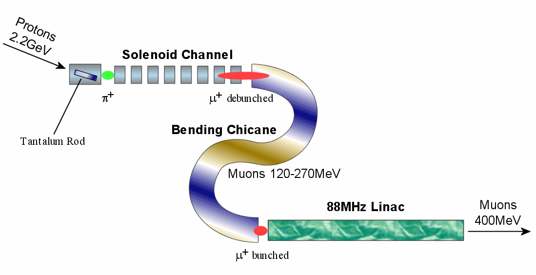
Current simulations focus on the proposed design in which the pion source is a tantalum rod (20cm long, 1cm in radius) being hit by a 2.2GeV pulse of protons that is assumed to have a Gaussian longitudinal bunch shape with RMS one nanosecond. The first component in the muon capture apparatus is a channel of transverse-focussing solenoids, the first of which encloses the rod (although the axis of the rod need not be parallel to the axis of the solenoid). The lack of longitudinal focussing means that the particles with larger vz will work their way to the front of the bunch, which will have spread out somewhat by the end of the channel. With this in mind, the next component is a 'chicane' of specially-designed bending magnets, in which the faster particles will go on paths further to the outside of two opposing bends in the accelerator.
| Figure 1. Schematic of the RAL muon front end design. |
The design is such that muons emitted directly down the solenoid channel with energies in range 120-270 MeV are meant to take an equal amount of time to get to the end of the bends. This means that they are re-bunched longitudinally at that point, ready to be accepted into the third component of the design, an 88MHz linear accelerator (not yet simulated).
These components constitute a muon front end for the Neutrino Factory, with bunched muons leaving the system with a mean kinetic energy of 400MeV. Other front end designs use different combinations of techniques to achieve the same output, for instance by using muon 'cooling' or several stages of linac acceleration.
Note that space-charge effects are negligible in these simulations, which simplifies the calculation considerably.
This is done using a fourth-order Runge-Kutta (RK4) solver for each particle in the (x,y,z,vx,vy,vz) phase-space, all coordinates being relative to the lab frame. A time-step was chosen by running batches of test particles through the solenoid channel and comparing the final positions with those obtained by halving the timestep. With the 10-picosecond steps used in the real simulations, it is estimated that after 120 nanoseconds (approximately the total time the beam is simulated for), no errors in position of a particle will be more than 2.5mm, with RMS and mean errors 0.5mm and 0.3mm respectively. This compares favourably with the size of the beam, which is typically at least 100mm across.
The way that forces are applied to the particles is special-relativistic and also fully integrated with the RK4 solver. RK methods in general solve first-order differential equations, whereas equations of motion are second-order in normal space. However, we find that the first time-derivative of the position in phase-space (d/dt)(x,v) = (v,dv/dt) is a function only of the original phase-space vector (x,v) - and possibly t, in the case of varying fields such as RF cavities. The calculation of dv/dt is complicated as usual by the relativistic mass-increase, but eventually one can derive the formula dv/dt = (F−c-2(F·v)v)/m0g, where F is the force as measured in the lab frame, i.e. e(E(x)+v×B(x)). These formulae are used in the program whenever the RK4 solver requests an evaluation of the derivative at some place in phase-space.
Currently the B-field contribution from solenoids is calculated using an analytic solution to Maxwell's equations with cylindrical symmetry, which yields the field as the sum of an infinite power-series. An error analysis similar to that used for determining the RK4 timestep was done, which revealed that truncating this series at the cubic term gives maximum and RMS positional errors of 0.25mm and 0.01mm respectively, so including any higher terms would slow down the simulation with no significant gain in accuracy.
The decay of pions is a random process in time, and the muon is emitted in an isotropically random direction in the rest frame of the original pion. Both of these factors would be better suited to a regime in which probability-density functions fp(x,v), fm(x,v) of phase-space are simulated, rather than being sampled discretely by macro-particles. While research on such Vlasov solvers is in progress, successful simulation of a 6D phase-space with reasonably high grid resolution has not been achieved.
Current simulations have taken the naďve approach of treating the macro-particles as actual particles and allocating each one a particular decay-time (and direction) as a function of the random number generator. Unfortunately this makes the simulation non-deterministic and produces considerable fluctuations in the predicted muon capture between one simulation and the next. This was not a severe limitation in the decay-channel-only optimisation, as the number of muons retained was some 25× as large as the random variations, but with the bending chicane added, the muon transfer fell to the level where these variations were beginning to confuse the optimiser.
When the longitudinal beam profile is calculated, there needs to be some mechanism to simulate that the original proton pulse is not instantaneous. This is done by simulating several (usually 5) copies of the initial pions, but with the release of any one pion delayed by a random amount of time taken from the normal distribution t~N(m=5ns,s=1ns). In cases where only the number of particles retained is important, all the particles may leave the source simultaneously, as without space-charge they do not interact. (They may also be simulated individually).
The simulation must take account of the various components situated in and around the beamline through which particles cannot pass. One of these is the rod source itself; others are the regions outside solenoids and the rectangular apertures of the bending magnets. Care must be taken that while ruling out particles that pass outside say, a solenoid, by a few inches, particles in a different part of the beamline intersecting the same plane (and thus technically 'outside' the solenoid) will not be removed. If this is implemented wrongly, particles can make false collisions with components.
After each run of the simulation, the result can be appended to a text file in the two-line format shown below.
zsrc=584;rotsrc=080;d1l=322;s2f=997;s3f=883;s4f=577;snf=490;alt=415;narrow=658;na1=422;na2=962;na3=474;
2.060580 (20936 particles) [v4.11] {E416DD6E}
The first line contains a list of named parameters that determine the accelerator design within the range being considered in the current optimisation. These have normalised values from 000 to 999, which can be rescaled onto the feasible range for that design parameter to find the actual value used. They may also be used to switch between different schemes of designs - for instance, the 'narrow' parameter is used to switch between four different algorithms for varying the solenoid radii along the decay channel.
The second line starts with the 'score' for the accelerator. From the optimiser's point of view, this just has to be a valid floating-point value with larger values corresponding to better designs (e.g. percentage efficiency). The rest of the line shows the number of particles used, the version number of the simulation software and a checksum of the beamline design file (a comment may also be added). This information is useful for distinguishing relevant results from those generated under different conditions or earlier (perhaps incorrect) versions of the software.
Optimisers are often implemented with steepest descent or hill-climbing algorithms that use the derivative of the score with respect to the parameters to determine which direction the optimiser will search along next. Unfortunately effects from pion decays make the score from the current simulations too variable at any fixed design for a derivative to be accurately calculated.
Instead, the optimiser uses an idea based on genetic algorithms (GAs). A conventional GA starts by running a number of random designs (the first generation) and produces a new generation using combinations of features from the best in the previous one (plus a small amount of random 'mutation'). This process is repeated until the score no longer increases. That would be far too wasteful for the purposes of this simulation, however, as it throws away the results from each generation after it generates the next (and a single simulation takes several minutes). Instead the optimiser logs all of the designs simulated (good or bad) to a file, and chooses a new design based on that data.
When the number of records in the file is small (e.g. less than 10), the program simulates a random design. Otherwise, it chooses one of the following four options with equal probability.
Since the results from independent optimisations are all still valid, this optimiser can be deployed as a distributed computing project, with near-independent calculations being made on many different machines. This resulting project status page is currently at http://stephenbrooks.org/muon1v4.html. Occasionally a "best results" or "cumulative results" file for the whole project is made available so that those who download it can base their optimisation on results found by other computers.
Before work on these simulations started, the muon front end had been developed [Grahame Rees] using standard modelling codes such as TRACE3D and Parmila. The basic design was as follows.
| Element S = Solenoid, D = Drift space | Length (m) | Field (T) | Aperture Radius (m) |
| S1 | 0.4066 | 20.0 | 0.1 |
| D1 | 0.5718 | ||
| S2 | 0.4 | -3.3 | 0.3 |
| D2 | 0.5 | ||
| S3 | 0.4 | 4.0 | 0.3 |
| D3 | 0.5 | ||
| S4 | 0.4 | -3.3 | 0.3 |
| D4 | 0.5 | ||
| S5 | 0.4 | 3.3 | 0.3 |
| D5 | 0.5 | ||
| S6-D23 | 9 more repeats of the above block | ||
| S24 | 0.4 | -3.3 | 0.3 |
| D24 | 0.5 | ||
| S25 | 0.4 | 3.3 | 0.15 |
| D25 | 0.5 | ||
| S26 | 0.4 | -3.3 | 0.15 |
| D26 | 0.5 | ||
| S27-D34 | 4 more repeats of the above block | ||
The tantalum rod pion source is positioned concentric with S1 and rotated by 0.1 radians about the Y-axis. The rotation is so that the pions, which tend to travel in helices within the solenoid, are not so likely to reimpact the rod. The results from one preliminary simulation to determine the effect of rod angle on muon transfer are graphed in figure 2.
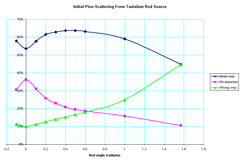
| Figure 2. How rod angle affects the performance of S1. |
This simulation was made with only the solenoid S1 in place, so the 'beam kept' figure counts the particles emerging from the correct end of this solenoid and 'wrong way' counts those from the opposite end. The graph suggests that a rod angle of ~0.45 radians would produce the lowest loss and avoid high re-interaction between the emitted particles and the rod.
| Name(s) | Description | Range of values | Notes |
| zsrc | Z-displacement of the rod source | -0.15 to +0.15 metres | Measured as the position of the centre of the rod relative to the centre of S1. |
| rotsrc | Rotation of the rod source about the Y axis | 0 to 0.5 radians | |
| d1l | Length of drift space D1 | 0.5 to 0.6 metres | The drift spaces in this area of the accelerator are primarily determined by other instrumentation, but this one can be varied slightly. |
| s2f s3f s4f | The strength of solenoids S2, S3 and S4 | ±2.5 to ±5.0 tesla | The sign as well as the strength can be changed by the optimisation; very low fields are not worth considering. |
| snf | Magnitude of field in solenoids S5-S34 | ±2.5 to ±4.0 tesla | S5's field has the same sign as this. The fields in later solenoids will have the same magnitude but sign controlled by alt. |
| alt | Controls how the solenoid fields S6-S34 change sign | Discrete; two values | Either the solenoids alternate in sign (+-+-+-), or they alternate in groups of five (+++++-----+++++-----). |
| narrow | Method of narrowing the solenoids S10-S30 | Discrete; four values | The solenoids narrow from 30cm to 15cm radius in one step; two steps via 22.5cm; three steps via 25cm, 20cm; or continuously in a section of linearly-decreasing radii. |
| na1 na2 na3 | Solenoid narrowing points | Solenoid number; integer from 10 to 30 | These control the points at which the step-narrowings take place, or where the linear narrowing begins and ends. na2 and na3 may be unused. |
The highest-scoring result recorded in this optimisation was the following.
| Parameter(s) | Value(s) |
| zsrc rotsrc | -0.01006 metres, 0.03253 radians |
| d1l | 0.5172 metres |
| s2f s3f s4f | +4.970, +4.660, +3.849 teslas |
| snf alt | +3.985 teslas, signs alternate in groups of five solenoids (+++++-----+++++ etc.) |
| narrow na1 na2 na3 | Solenoid radii decrease in three steps: to 25cm at S10, 20cm at S13 and to 15cm at S30. |
This was given a score of 7.066% muon transfer, but due to statistical effects introduced by the pions (and the fact this was the best result, so likely having an upward fluctuation), the true figure is probably to be closer to 6.5%. The total weight of the initial pions was 14617.2, which corresponds to 105 protons impacting the rod, so the efficiency at the end of the decay channel is 6.5% of 14617.2, or about 950 m+ per 105 p+ on the target (m+/p+ = 0.95%).
Unlike the preliminary simulations, the optimisation of the full decay channel seemed to favour small rod rotation angles, perhaps because capture of the pions by S2 and S3 is more difficult when the rotated rod produces a larger X-axis spread of particles. The tendancy towards choosing the strongest possible focussing solenoids for the majority of the beamline is not surprising given that the goal is to minimise beam loss, however the low value of s4f suggests a higher field at that point might not be beneficial.
The second main optimisation, which is still under study, varies the solenoid channel in the same way as before but also tracks the particles through the second segment of the design. The score for each design is calculated from the number of particles retained at the end of this second part, meaning that although the bending chicane itself cannot be modified here due to beam optics considerations, the decay channel can be optimised in such a way as to be most compatible with it.
The bend consists of four identical 'triplets' of magnets (B1, B2, B1) with fields such that a pencil beam of muons with varying energies emerges from a triplet as a dispersed beam and rotated by 101°. When that dispersed beam enters a second triplet at the correct angle, it is turned back into a pencil beam (up to the correctness of the field within the magnets) but by then the higher-energy muons will have travelled further, giving the slower ones time to catch up. To cancel the dispersion produced by the decay channel, 404° of bends are needed, so to avoid layout problems the second pair of triplets bends in the opposite direction.
Figure 3, produced using the same tracking code as used for the optimisation, shows how the magnets will bend the paths of muons with energies of 120 MeV (red) up to 270 MeV (violet) in steps of 10 MeV.
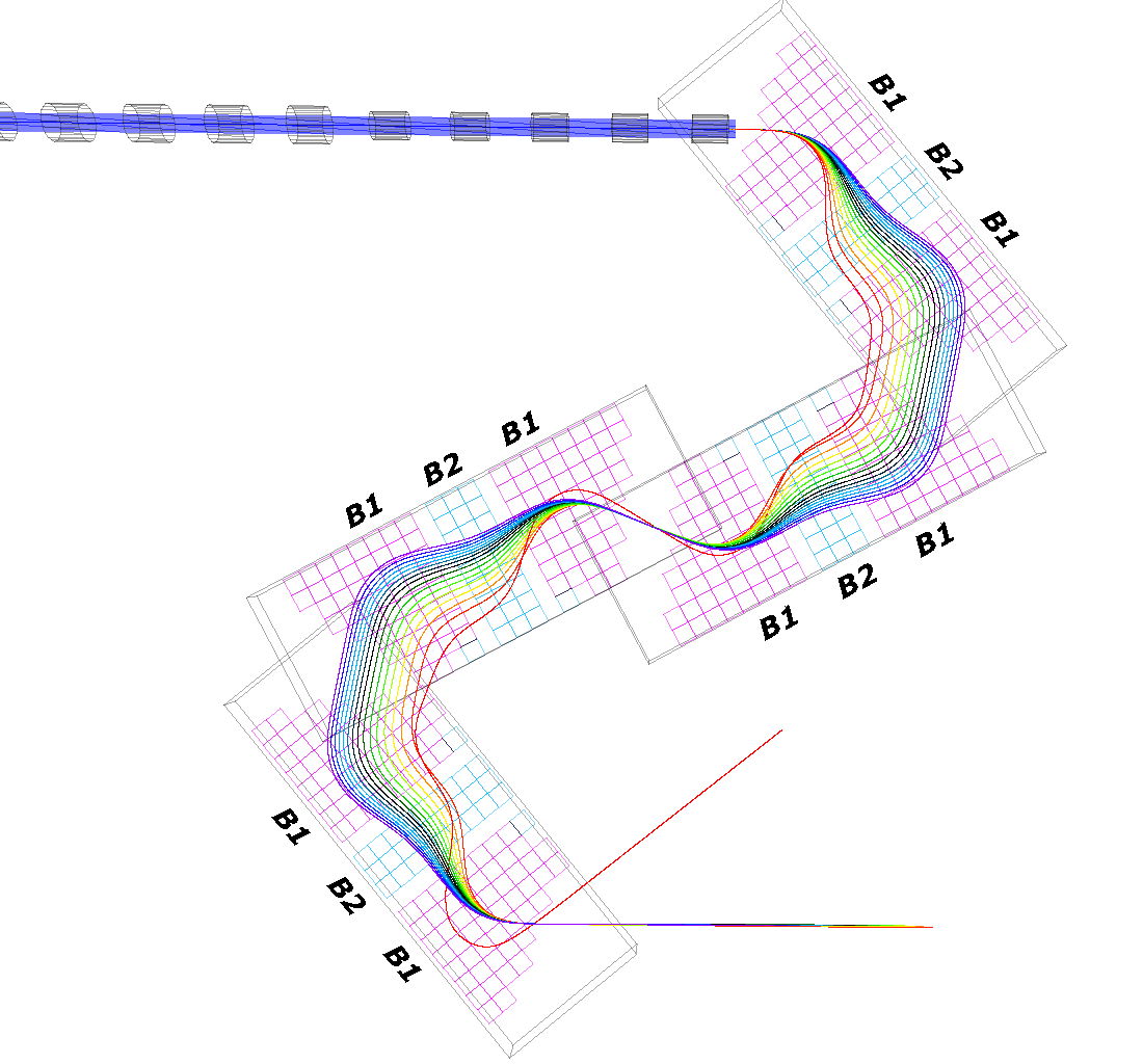
| Figure 3. The reverse phase slip bending chicane in action. |
A preliminary simulation calculated the distribution of muon arrival times at the end of the bending chicane, to see if the beam will be sufficiently bunched to be accepted into the 88MHz linac.

| Figure 4. Longitudinal beam profile upon re-bunching by the chicane. |
As figure 4 shows, the bunch emerging from the chicane is approximately the same length as the linac bucket (an 88MHz wavelength is shown for comparison). Some loss of the distribution tails will occur.
Before the optimisation, the optimal design for the decay channel was run with the bending chicane simply added onto the end. It produced a muon yield of 1.878±0.027% m+ per p+ emitted from the source, where the figure quoted is a 95% confidence interval based on repeated runs of the simulation to reduce statistical effects. After the combined optimisation using the number of muons at the end of the chicane as the score, the best design had a yield of 1.930±0.013%. This is higher by a statistically significant amount, although doubts about the optimiser's performance when large statistical fluctuations are present in the scoring mean this may not be the highest possible figure. It corresponds to a ratio of m+/p+ = 0.28%.
The objectives in each section here are listed with the most urgent or immediately practical first and the furthest-off or most difficult to implement last.