Quantitative Optimisation Studies of the Muon Front-End for a Neutrino Factory

Stephen Brooks (sb@stephenbrooks.org)   June 2004
1.  Abstract

In a Neutrino Factory, short proton pulses hit a target, producing pions at widely varying angles and energies.  Efficient pion capture is required to maximise the yield of decayed muons, which proceed via acceleration stages into a muon storage ring to produce neutrinos.  This paper presents optimisation of a solenoidal decay channel designed for high-emittance pions, based on schemes from CERN and RAL.  A non-linear tracking code has been written to run under an optimisation algorithm where every beamline element can be varied, which is then deployed as a distributed computing project.  Some subsequent stages of muon beamline are also simulated, including RF and non-RF phase-rotation techniques and in one option, initial muon acceleration to 400MeV.  The objective is to find optimal transmissions for each front-end concept.

2.  Design Method
2.1.  Tracking Code

The high-divergence beam in the decay channel favours a fully three-dimensional simulation, since this will implicitly include all dynamical nonlinearities appearing from large particle angles and energy deviations.  Previous concept work [1] was done using linear transport in the code PARMILA.  The new code is called Muon1. A particle's position and velocity (in the laboratory frame) can be combined into a phase-space vector s = (x,y,z,vx,vy,vz).  A first-order differential equation expresses ds/dt in terms of s, t and other knowns such as the applied magnetic fields and describes the future path of the particle.  This is solved numerically using the fourth-order Runge-Kutta method with timestep δt = 0.01 ns, chosen empirically by observing the results of tracking with different values.  Solenoid B-fields are calculated from a third-order expansion in (r,z).

The decay of π+ to μ+νμ (π+ mean life = 26.033 ns) requires the tracking code to treat decays properly as well, since both the mass of the particle and its momentum change due to the kick from the outgoing νμ.

2.2.  Optimisation System

Placement of components and drift spaces to form a beamline is controlled by 'lattice files,' which specify the parameters (field strength, length, etc.) of each.  For optimisations, a Muon1 lattice file can define a whole space of designs to be investigated.  In this case, the beamline generated is a function of both the lattice file and a 'genome,' which specifies a single design in the space by showing where each non-fixed parameter should be set inside its allowed range.

The terminology is inherited from the field of genetic algorithms, as the results of many simulated designs from a space can be considered a 'gene pool,' from which better-performing individuals can be selected to base future designs on.  Performance is measured by the percentage of particles reaching the end of the beamline when the design is run with the tracking code.  Sometimes particles are only counted within a specified energy range.

The production of new designs can now be automated.  'Mutation' steps take a single good design and change one or several of its parameters by a random amount, to search the nearby space for better designs.  'Crossover' and 'interpolation' steps take two previous good designs and combine them either by interlacing their parameter values, or linearly interpolating between them.  Recently, other types have been added to improve performance, including one that ascends along an approximation to the local gradient.  If the optimiser has very few previous designs to learn from, it will simulate completely random ones to sample the space initially.  As the scoring includes stochastic effects from the finite number of particles and their decays, the gradient cannot be computed by the standard method of making small changes to every parameter (there are also a prohibitively-large number of parameters).  So instead it is calculated from a linear regression of the existing data on a region of finite size.

Given lattice files defining the design spaces of interest, the system may now be run in 'closed loop' mode.  Taking advantage of this, the properly configured code was made available from a website [2] and an FTP procedure added that uploads results produced on any participating computer to the central database.  Samples of better designs from the entire project can be downloaded to individual computers, making the exchange two-way, so that the set of computers running the program behaves as a large parallel optimiser.  Volunteers to run the code were abundant and the project now uses several hundred PCs.

3.  Pion Decay Channel

Particles are captured from the target in a series of superconducting solenoids, used because they can achieve a high focussing field over a wide aperture (e.g. 4 T over an 80 cm diameter bore).  The pion distribution was calculated using LAHET [3,4] for a 2.2 GeV proton beam hitting a 2 cm diameter, 20 cm-long tantalum rod.  This rod is enclosed within the first solenoid, which has the highest field and a smaller bore than the rest.  The rod is tilted to prevent pions reimpacting after one revolution of a Larmor helix.  The entire channel has a length of 30 m since this corresponds to roughly 2½ pion decay times.  Transverse RMS emittance at the end of the first solenoid is roughly 13000π mm mrad, reducing to 6250π mm mrad at the end of the channel through collimation losses.

The original design has the structure in Table 1, with the rod tilted by 0.1 radians and centred in solenoid 1.  Tracking gave it an efficiency of 3.1% of a particle retained per original pion emitted (efficiencies will be quoted in these units from now on).

Table 1.  The original decay channel lattice.
Element NumberSolenoid Field (T)Solenoid Radius (m)Solenoid Length (m)Drift Length (m)
1200.10.40660.5718
2-3.30.30.40.5
34
4-24-3.3, 3.3†
25-340.15
† Alternates in sign: negative in even-numbered elements.

This was generalised to an optimisation range with 12 degrees of freedom, as follows.  The rod can be displaced up to 15 cm along the axis of the solenoid and tilted by anything from 0 to 0.5 radians.  The first drift can be from 0.5 to 0.6 m long.  Solenoids 2-4 can be from 2.5 to 5 T with the upper limit reducing to 4 T for the rest.  Their polarity can either alternate (as before) or change every fifth cell.  Bore narrowing takes place from cells 10 to 30 via one, two or three equal decrements, or a linear tapering, all controlled by additional optimiser variables.

The optimisation gave a maximum efficiency of 6.5%, mainly by selecting the largest allowed fields and apertures, but with the interesting features of preferring the solenoid signs in groups of five and having a significantly sub-maximal field value for solenoid 4.

Next, a more ambitious optimisation of ~137 variables was attempted, in which all solenoid parameters were allowed to vary independently (see Table 2).

Table 2.  Ranges for generalised solenoid channel.
Element NumberSolenoid Field (T)Solenoid Radius (m)Solenoid Length (m)Drift Length (m)
10-200.10.2-0.450.5-1
2-4-5 to +50.1-0.40.2-0.6
5+-4 to +4
Final0.15N/A

Efficiencies of up to 10.3% were produced from this, although the imposition of a 15 cm radius at the end of the channel has just made the optimiser produce a betatron focus there.  It also chose the minimal solenoid length so that pions with high-angle trajectories could get through.  Removing that constraint allows yields of up to 16.1%, though the need to optimise jointly with subsequent stages of the accelerator is becoming clear, as otherwise the highest raw transmission is achieved at the expense of the usefulness of the beam.

As was hinted in the 12 parameter optimisation, the design contains a 'matching' section near the beginning (see Table 3).  Presumably this manipulates the beam shape into something more suited to the maximised regular focussing used later in the lattice.  This is not an artefact of non-convergence of the optimiser, since when the asterisked parameters are altered to be maximal the transmission efficiency reduces from 10.3% to 8.5%.

Table 3.  Matching section in the optimal decay channel.  Asterisked values deviate significantly from using the largest possible solenoids and the shortest possible drifts.
Element NumberSolenoid Field (T)Solenoid Radius (m)Solenoid Length (m)Drift Length (m)
1200.10.450.5
250.3514*0.60.5
350.40.423*0.5
44.189*0.40.3806*0.6612*
550.40.5299*0.5075
63.824*0.40.60.5170

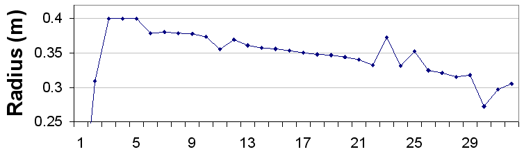
Notably, all the solenoid fields now have the same sign: this can be seen as an extrapolation of the 12 parameter run in which alternation in blocks was preferred over changing every solenoid.  Further investigation found a physical reason why the assumption of alternating fields in the original design was wrong (see Figure 1).  The off-energy particles in the alternating-field channel suffer a transverse displacement every two cells, meaning they gradually move out of the solenoid apertures.  In a non-alternating channel, their transverse orbits just precess.

Figure 1.  Transverse orbits of off-energy particles in alternating solenoidal channels (top) and non-alternating ones (bottom).
Figure 1.  Transverse orbits of off-energy particles in alternating solenoidal channels (top) and non-alternating ones (bottom).
4.  Phase Rotation Using Chicane
Figure 2.  Longitudinal phase space before the chicane (left; remaining pions shown in green) and after it (right).
Figure 2.  Longitudinal phase space before the chicane (left; remaining pions shown in green) and after it (right).

Described comprehensively in [1], the chicane provides a reverse shear in longitudinal phase space (see Figure 2) to counteract the drift through the decay channel, yielding a bunch short enough to be inserted into a linac.  It uses the dispersion from large-angle bending magnets to give high-energy particles longer paths ([1], fig. 3) so that low-energy particles can catch up.  The bending field varies nonlinearly across the aperture to synthesise the correct path lengths.  Thus Muon1 uses an OPERA-3d field map from the work described in [5] for its tracking.

This (fixed) chicane was appended to both the 12- and 137-parameter decay channel optimisation ranges.  The fixed-radius solenoid at the end of the decay channel was removed so the chicane would dictate the acceptance to optimise for; the results are shown in Table 4.

Table 4.  Results from the chicane optimisation.
Efficiencies at:Original12-param137-param
Decay channel3.1%6.5%10.3%
End of chicane1.13%1.93%2.64%
Separately optimisedN/A1.88%2.00%

As expected, the separately-optimised decay channel transmits fewer particles through the chicane than the one optimised jointly with the chicane.

The optimal design for 137 parameters is less trivial than that for the decay channel alone.  Elements in the central section still have minimal drift length and maximal field, but the solenoid radii assume a slowly narrowing pattern (Figure 3).  The exact origin of this is unknown, though it must be related to the solenoid end-fields, as the linear part does not depend on the radius.

Figure 3.  Narrowing of the solenoid radii.
Figure 3.  Narrowing of the solenoid radii.

The solenoid lengths were optimised to a value in the interior of the allowed range, with median 0.463 m.  Examining regular solenoid channels using linear optics gives the helical rotation within each solenoid as

θ =
qBzLsolenoid
m0γvz
,

where m0 and q are the rest mass and charge of a particle with relativistic factor γ and the on-axis solenoid field is Bz.  If θ is too small, the particles take many repeats of the focussing structure to return to their original orientation, moving in a very large loop in transverse space and likely to be lost in the process.  The solenoid-drift focussing is also only conditionally stable: eigenvalue analysis of the transverse mapping matrix shows that

Ldrift
Lsolenoid
4
θ
 
sin θ
1−cos θ
+
2
1−cos θ
 

is required for the orbits to remain bounded.  From this, we must have θ<192° for the optimised lattice to be stable.  The chicane is designed to transmit muons with an energy range of 120 to 270 MeV, which in this lattice have θ values of 160° to 88°, staying well inside the stable region and keeping the transverse paths compact.

The beam entering the chicane has a transverse RMS emittance of 8870π mm mrad and a longitudinal one of 0.89 eV s (insofar as one can fit an ellipse to the banana-shaped phase space).  Leaving the chicane, the transverse planes differ, with εx=9300 and εy=2230 mm mrad.  The RMS half-duration of the output bunch is just 1.52 ns with a longitudinal emittance of 0.075 eV s: not much longer than the proton bunch hitting the target (pions were released at a spread of times with standard deviation 1 ns).

5.  Muon Linac to 400MeV

After the chicane is a linear accelerator using 88MHz RF cavities and the same solenoidal focussing structure as in the decay channel.  This has not yet been optimised, but the baseline design has 90 RF cavities with a gap voltage of 3.6 MV, operating at phases such that the output energy of the beam is 400±100 MeV.

Figure 4.  Phase space at end of muon linac.
Figure 4.  Phase space at end of muon linac.

Figure 4 shows the result of simulating this design appended to the optimal chicane.  Not all of the beam has stayed within the bucket: the amount in the desired energy range is 1.36%, where a total of 1.57% was transmitted.

6.  Alternative RF Phase Rotation
Figure 5.  Phase space at end of phase rotation.
Figure 5.  Phase space at end of phase rotation.

This approach uses a beamline of 31.4 MHz cavities and solenoids placed directly after the decay channel.  They compress the energy range down to 180±23 MeV in preparation for injection into a muon cooling ring.  The baseline design uses 30 cells with a gap voltage of 2.25 MV; this was simulated in Muon1 and Figure 5 shows the output phase space.

The efficiency into the required energy range is 1.70% and 3.81% is transmitted in total.

7.  Summary

The applicability of optimisation with a large number of parameters has been demonstrated on a practical accelerator design problem.  Holistic optimisation, where many components are optimised together while being tracked end-to-end, appears to have an advantage over separate optimisation, particularly at higher numbers of parameters.

8.  Future Work

Quantitative optimisation of the linac and the alternative RF phase rotation design involving is already underway.  The cooling ring that the phase rotation section injects into will be optimised jointly with it later on.

A.  References

[1] G. H. Rees et al., "Muon front-end chicane and acceleration," J. Phys. G 29 (2003) pp. 1673-1677.
[2] http://stephenbrooks.org/muon1.
[3] Richard E. Prael and Henry Lichtenstein, "User Guide to LCS: The LAHET Code System", LANL report LA-UR-89-3014, Revised (1989).
[4] LAHET dataset generated by Paul Drumm.
[5] M. R. Harold, "Magnets for a Muon Front End Chicane," NuFact02 conference proceedings.